Contrastive Multimodal Fusion with TupleInfoNCE

Traditional representation learning for multimodal data focuses either on contrasting different modalities to maximise mutual information or concatenating all modalities and then contrast across these combines tuples. The fomer approach fail to learn the complementary synergies across modalities and the latter one tends to neglect the weaker modalities.

This paper propose to “contrast multimodal input tuples”, making those describing the same scene closer and those from different scenes fall apart. In order to avoid the ignorance of weaker modalities, more challenging negative samples are needed.

The core idea of paper is: strong variations between positive and anchor samples = smaller MI but greater degree of invariance against nuisance variable (tradeoff)

infoNCE loss

Given a positive sample $x_{2,i}$ and negative samples $x_{2,j}$ of an anchor variable $x_{1,i}$, InfoNCE loss is: \(\mathcal{L}_{\text{NCE}} = -\mathbb{E}[\log\frac{f(\boldsymbol x_{2,i},\boldsymbol x_{1,i})}{\sum_{i=1}^Nf(\boldsymbol x_{2,j},\boldsymbol x_{1,i})}]\) A multimodal input is a K-tuple: $\boldsymbol t = (\boldsymbol v^1,\boldsymbol v^2,…,\boldsymbol v^K)$, where $\boldsymbol v^k$ is one modality.

Anchor samples $\boldsymbol t_{1,i}\sim p(\boldsymbol t_1)$ are drawn as well as positive examples $\boldsymbol t_{2,i}\sim p(\boldsymbol t_2 \vert \boldsymbol t_{1,i})$ and negative samples $\boldsymbol t_{2,j}\sim p(\boldsymbol t_2)$.

Maximising the mutual information between $t_1$ and $t_2$ can ignore the weak modality and sacrifice the synergy, when $\boldsymbol v^k$ is the dominating modality such that $I(\boldsymbol v^k_2,\boldsymbol v^k_1)»I(\boldsymbol{\bar v}^k_2,\boldsymbol{\bar v}^k_1)$.

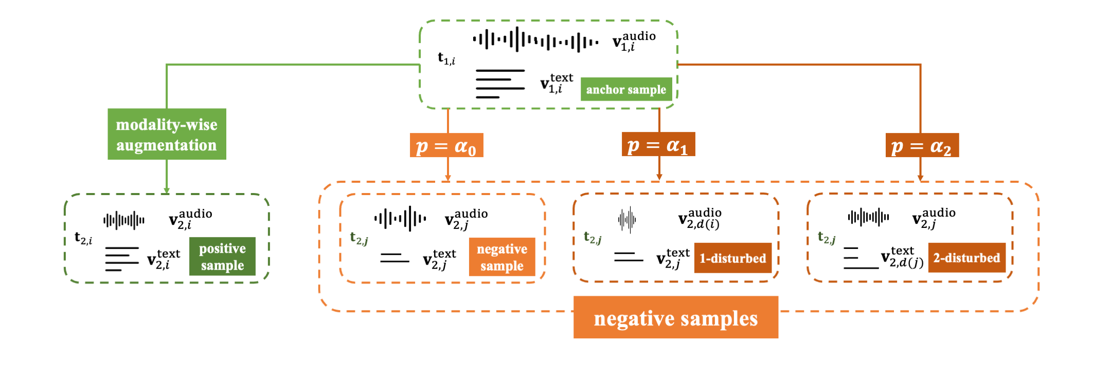
To allieviate the limitation, the paper propose a novel tuple disturbing strategy to generate challenging negative samples: only substitute one modality $\boldsymbol v^k_{2,d(j)}$ in the tuple with the modality from another scene. This keeps the disturbed negative example similar to positive one other than $\boldsymbol v^k_{2,d(j)}$. The goal for the network is to distiguish this modality from others.

The object of TupleInfoNCE is to fusing the multimodal input $\boldsymbol t = (\boldsymbol v^1,…,\boldsymbol v^K)$. Given an anchor sample $\boldsymbol t_{1,i}\sim p(\boldsymbol t_1)$, the positive sample $\boldsymbol t_{2,i}\sim p_\beta(\boldsymbol t_2\vert \boldsymbol t_{1,i})$ is drawn. And each negative sample $\boldsymbol t_{2,j}\sim p(\boldsymbol t_2)$ is sampled from another scene with probablity $\alpha_0$ or is sampled from $p(\boldsymbol{\bar v}^k)p(\boldsymbol v^k)$ as a k-disturbed negative sample with the probability of $\alpha_k$. Note that $\sum_{k=0}^K\alpha_k = 1$.

The strategy can be visualized as the following procedure:

So the loss function of TNCE is:

\[\mathcal{L}_{\text{TNCE}}^{\boldsymbol{\alpha\beta}} = -\mathop{\mathbb{E}}\limits_{\boldsymbol t_{2,i}\sim p_\beta(\boldsymbol t_2\vert \boldsymbol t_{1,i})\\ \boldsymbol t_{2,j\vert j\neq i}\sim q_\alpha(\boldsymbol t_2) }[\log(\frac{f(\boldsymbol t_{1,i}, \boldsymbol t_{2,i})}{\sum_jf(\boldsymbol t_{1,i},\boldsymbol t_{2,j})})]\]

where the distribution $q_\alpha(\boldsymbol t_2) = \alpha_0 p(\boldsymbol t_2)+\sum_{i=1}^K\alpha_ip(\boldsymbol{\bar v}^k)p(\boldsymbol v^k)$

evaluation and optimization challenge

Evaluation: use cross modal discrimination as a surrogate task, which looks for the $\boldsymbol{\bar v}^k $ by $\boldsymbol v^k$.

From a validation set $t_1,…,t_M$, given any augmented $\boldsymbol v’^k_n\sim p_{\zeta_k}(\boldsymbol v’^k\vert \boldsymbol v’^k_n)$, find its corresponding rest modalities $\boldsymbol{\bar v}^k_n$.

We compute the probability that the corresponding rest modalities of $\boldsymbol v’^k_n$ is $\boldsymbol{\bar v}^k_l$ as:

\[p^k_{nl}(\boldsymbol {g^{\alpha\beta}})=\frac{\exp(\boldsymbol{g^{\alpha\beta}}(\boldsymbol v'^k_n)\cdot\boldsymbol g^{\alpha\beta}(\boldsymbol{\bar v}^k_l)/\tau)}{\sum^M_{m=1}\exp(\boldsymbol g^{\alpha\beta}(\boldsymbol v'^k_n)\cdot\boldsymbol g^{\alpha\beta}(\boldsymbol{\bar v}^k_m)/\tau)}\]

where $\boldsymbol g^{\alpha\beta}(\cdot)$ is the optimal multimodal encoder and $\tau$ is the temperature parameter.

And the accuracy for the $k^{th}$ modality is formulated as:

\[\mathcal{A}^k(\boldsymbol g^{\alpha\beta})=\sum^M_{n=1}\mathbb{I}(n=\arg\mathop{\max}_{l}p^k_{nl}(\boldsymbol g^{\alpha\beta}))/M\]

And the ultimate reward can be written as:

\[\mathcal{R}(\alpha)=\sum_{k=1}^K \mathcal{A}^k(\boldsymbol g^{\alpha\beta})\]

Optimization:

\[\begin{aligned} \text{maximize } &\mathcal{R}(\alpha)=\sum_{k=1}^K \mathcal{A}^k(\boldsymbol g^{\alpha\beta})\\ \text{s.t. } &\boldsymbol g^{\alpha\beta}=\arg\mathop{\min}_{\boldsymbol g} \mathcal{L}^{\alpha\beta}_{\text{TNCE}}(\boldsymbol g) \end{aligned}\]

which is a standard bilevel optimization where $\alpha$ and $\boldsymbol g$ can be optimized alternatively in a single training pass. The restriction $\sum_{k=0}^K\alpha_k=1$ is relaxed and $\alpha$ is initialized with $\mathcal{N}(\mu_0,\sigma I)$.

During each epoch $t$, $\alpha_1,…,\alpha_B$ is sampled from $\mathcal{N}(\mu_t,\sigma I)$, and $g^1_{t+1},…,g^B_{t+1}$ are trained correspondingly, and then $\mu$ is updated with the formula:

\[\mu_{t+1} = \mu_t+\eta\frac{1}{B}\sum^B_{i=1}\mathcal{R}(\alpha_i)\nabla_\alpha\log(p(\alpha_i;\mu,\sigma))\]