Brief Introduction to Active Learning

Active Learning happens when we don’t have the time and energy to annotate all datas so we want to annote those samples which will improve our models the most. Usually there are two heurestic ways to pick such samples iteratively until we reached the budget of total annotations.

• Uncertainty sampling: we give the sample which the model is most uncertain about the highest rank, namely, we annotate the sample that the model isn’t sure about first. There are a few methods to measure the uncertainty:

  1. Add the sample with the highest entropy of prediction result to annotation set, namely take $x$ such that: \(x = \arg\max_x H(p_x) = \arg\max_x -\sum_{c\in C} p_x^c \log_2(p_x^c)\)

  2. one variant of 1. is using the variation ratio $1- \max_{c\in C} (p_x^c)$ as the criterion to rank the samples.
  3. another variant of 1. is using \(\max2_ip_x^i - \max_jp_x^j\), where $\max2$ denotes the second largest value. In other words, we pick the sample whose probability of the most probable class is the closest $j$ to that of the second probable class $i$.
  4. In SVMs we can use the distance between every sample and the hyperplane as the criterion, so we can pick the point closest to the margin as the next to annotate.

• Diversity sampling (Query by committee): instead of measuring uncertainty given by a single model, we infer each image with an ensemble of many models and find the one where the predictions vary the most among different models. Same as uncertainty sampling, there are two criteria to measure the diversity of the prediction:

  1. Pick the sample with the smallest difference between the result with the top most and second most votes from all models.

  2. Pick the sample with the maximum vote entropy from all models, namely pick $x$ such that: \(x = \arg\max_x - \sum_{c\in C}\frac{V(c)}{|C|}\log(\frac{V(c)}{|C|})\)

Some challenges of active learning in deep learning scenario are that 1. Multi-class classification networks with softmax are usually confident about the prediction result, which poses a challenge to uncertainty sampling; 2. it’s usually time and resource consuming to go one pass over the whole dataset, so instead of picking one sample at a time we prefer to select a batch, which is not trivial.

Self/Semi-supervised Learning for Data Labeling and Quality Evaluation

This paper suggests to “use contrastive learning methods to obtain an unsupervised representation of unlabelled data and construct an NN graph over data samples based on the representation.”

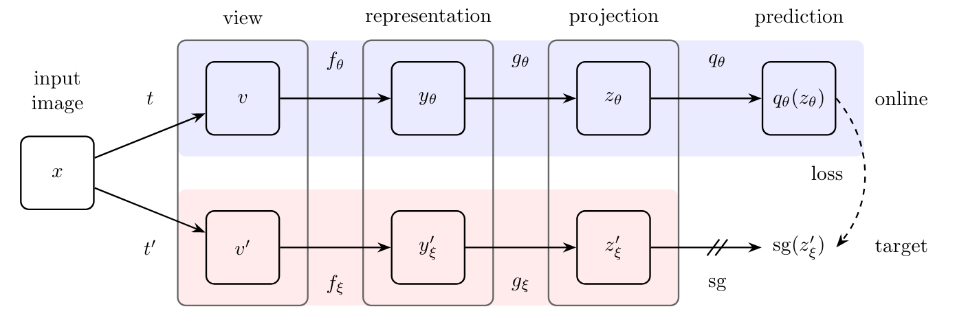
• contrastive learning for unsupervised representations

  the goal is to minimize: \(L_{\theta, \epsilon} = ||\bar{q_\theta} - \bar{z_\epsilon}'||^2_2\) where the $\bar{q_\theta}$ is the normalised prediction of the online network where $\bar{z_\epsilon}’$ is the normalized projection of the target network.

  

• NN graph

  after we learn the representation from the previous step, we propogate the label based on a NN graph, which is constructed based on the sparse adjacency matrix: \(W_{ij} = 1\{j\in NN(i,k)\}\cdot\exp(l(f_\theta(x_i), f_\theta(x_j)) / T)\) Where $T$ is a temperature parameter.

  Then the labels are propogate with the following rules: \(\hat{Y}^{(t+1)} = \hat W Y^{(t)} \\ Y_u^{(t+1)} = \hat Y_u^{(t+1)} \\ Y_l^{t+1} = Y_l^{(0)}\) where the subscript $u$ means unlabelled and $l$ for labelled, and $\hat W$ being the normalized counterpart of adjacency matrix $W$ given by $\hat W = D^{-1/2}WD^{-1/2}$.

Not All Labels are Equal

The second paper proposes to use an inconsistency-based acquisition function for ranking and a pseudo-labeling module to label the easy images. We will talk about these two techiniques separately.

• inconsistency-based acquisition function:

  instead of training an ensemble of many models, we can augment each sample. Assume that if the prediction result of a sample and that of its augmentation are similar, then the inconsistency of this sample is low, which means the model is robust for this sample, thus we can assign a lower rank for it.

  To express in a mathematical way, we can define the inconsistency of an image $\Delta$ and its augementation $\hat \Delta$ as: \(I(\Delta) = \max_i\{L_{con_C}(c_i', c_i)\}\) Where $L_{con_C}(c_i’, c_i)$ is defined over each pair of corresponding detection in the original image and augmentation by: \(L_{con_C}(c_i',c_i) = 1/2[KL(c_i',\hat c_i),KL(\hat c_i,c_i')]\) Similarly we can also define the uncertainty of the image (note that we don’t use the augmentation in this case) as: \(H(\Delta) = \max_i\{H(c_i)\}\) In the end, the acquisition score of $\Delta$ is: \(A(\Delta) = H(\Delta)\times I(\Delta)\)

• Pseudo-labeling to prevent distribution drift

  we can confidently label some samples when the predidtion confidence is above some threshold and use the labelling as ground truth for the next training cycle. The criterion of pseudo-labeling is: \(\hat y_i^p = 1, \text{if }p=\arg\max(c_i)\text{ and } c^p_i \geq \tau\) One minor issue with this method is that the model could be confident with one prediction in the sample but not the others, the paper suggests that we can tackle it by introducing a pseudo-label loss: \(L_{conf}(c, y, \hat y) = -\sum_{i\in Pos}\sum_{p=1}^{|c|}y_{ij}^p\log(c_i^p) - \sum_{i\in Neg}\log(c_i^0) - \sum_{i\in \hat {Pos}}\sum_{p=1}^{|c|}\hat y_{ij}^p\log(c_i^p)\)