Preliminary Knowledge

1. Mutual Information

Suppose we have $x$ and $y$, which are random variables. The entropy $H(xy)$ can be viewed as the # of bits to encode them together. From this definition, we can see that $H(xy) = H(x)+H(y)$ iff $x$ and $y$ are independent.

We define the mutual information(# shared bits used to reduce to independent generation) between $x$ and $y$ as follows:

$I(x;y)=H(x)+H(y)-H(xy) = \sum_{x,y}P_{xy}(x,y)(\log\frac{1}{p(x)}+\log\frac{1}{p(y)}-\log\frac{1}{p(x,y)})$

​ $=\sum_{x,y}P_{xy}\log_2\frac{p_{xy}(x,y)}{p(x)p(y)}$

Note that MI has the following properties ( $x$ and $y$ are symmetrical in formula):

1. $I(x;y)\geq 0$, with equality iff $x$ and $y$ are independent.

2. $I(x;y)\leq H(x)+H(Y)$, with equality iff both of $x$ and $y$ are constant and entropy are both 0.

3. $I(x;y)\leq \min\{H(x),H(y)\}$.

4. $I(x;y)=H(y)$ iff y is determined by $x$.

5. $H(y\vert x) = H(y)-I(x;y) = H(xy)-H(x)\geq 0$ is the conditional entropy of $y$ given $x$, but really an expectation $E_{x\sim X}[H(y\vert X=x)]$.

6. $H(xy)=H(x)+H(y\vert x)$, which is the chain rule of entropy.

7. $I(x;y) = H(y) - H(y\vert x) = H(x) - H(x\vert y)$.

2. KullBack Leibler Divergence

$P$ and $Q$ are defined on the same probability space, then the relatively entropy from $Q$ to $P$ is:

$D_{KL}(P\vert \vert Q) = \sum_{x\sim X}P(x)\log(\frac{P(x)}{Q(x)})$ for discrete probability distributio

$D_{KL}(P\vert \vert Q)=\int_{-\infty}^{+\infty}p(x)\log\frac{p(x)}{q(x)}dx$ for continuous variable

Note that the relatively entropy is always greater than 0.

So $\sum_{x}[p(x\vert y)\log p(x\vert y) - p(x\vert y)\log q(x\vert y)]\geq 0$,

where $\sum_x -p(x\vert y)\log p(x\vert y) = H(x\vert y)$ (definition of entropy).

$I(x;y) = H(x) - H(x\vert y) \geq H(x) + \sum_x p(x\vert y)\log q(x\vert y)=^{def}=\hat{I}(x,y)$ (MI’s $7^{th}$property),

here $H(x)$ is the entropy and $<\log q(x\vert y)_{p(x,y)}>$ is the energy.

3. Contrastive Predictive Coding

To get a thorough understanding of contrastive predictive coding, it is highly recommended that you read the paper yourself since this blog would only walk you through this topic briefly as a basis for InfoMax.

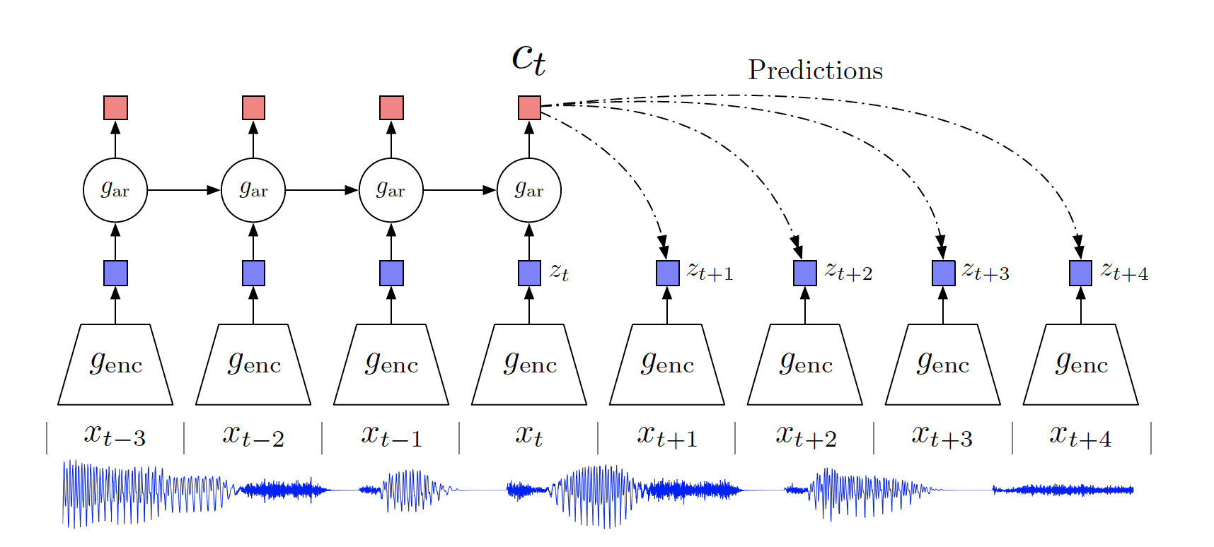
As in this figure, we use an encoder $g_{\text{enc}}$ to encode the raw data $x_t$ into a latent representation $z_t$ and an autoregressive model $g_{\text{ar}}$ to produce a context latent representation $c_t$ based on historical records of $z_{\leq t}$. In order to tell whether $g_{\text{enc}}$ can preserve useful information from the raw data, we want the representation vector $c_t$ to be a good predictor for the representation vectors $z_{t+i}$ for future input $x_{t+i}$.

To make $c_t$ a good predictor for $k$ future inputs, we optimize the encoder and the autoregressive model by constructing training example, where inputs from the same batch $x\in\{ {x_{1},…, x_N}\}$ are grouped into positive examples $<x_i,c_i>,i\in \{1,…N\}$ and negative training examples $<x_i, c_j>, i\in\{1,…,N\}, j\in\{1,…N\} \backslash i$.

Then we construct the loss function of $f(x_{t+k},c_t)$ as follows: \(\mathcal{L}_N = -\mathop{\mathbb{E}}\limits_{X}[\log\frac{f_k(x_{t+k},c_t)}{\sum_{x_j\in X}f_k(x_j,c_t)}]\)

4. MultiModal InfoMax

This paper proposed a framework MMIM, which hierarchically maximizes the MI in unimodal input pairs and between multimodal fusion.

previous work in learning unified representations:

1. Loss back-propogation: only tunes based on gradients
2. geometric manipulation in feature spaces: lack of control in information flow

Enhance two types of MI in representation pairs:

• between unimodal representations
• between fusion results and their low-level unimodal representations

downstream application: Multimodal sentiment analysis

Problem definition

input: unimodal raw sequences $X_m\in R^{l_m\times d_m}$, where $l_m$ is the sequence length and $d_m$ is the representation vector dimension of the modality $m$. Here we have $m\in\{t,v,a\}$

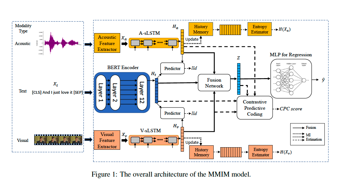
We use $h_t = BERT(X_t;\theta^{BERT}_t)$, $h_m = sLSTM(X_m;\theta^{LSTM}_m), m\in\{v,a\}$

use $I(x;y) = H(x) - H(x\vert y) \geq H(x) + \sum_x p(x\vert y)\log q(x\vert y)=^{def}=\hat{I}(x,y)$

to obtain: $I(X;Y) \geq H(Y) + E_{p(x,y)}[\log q(y\vert x)]$, denoted as $I_{BA}$

Treat text as $X$, other modalities as $Y$, in order to train a predictor $q(x\vert y)$ from higher dimensions $h_t$ to lower $h_m$ and use text as predominate modality.

Use multivariate Gaussian distribution $q_\theta(y\vert x)=N(y\vert \mu_{\theta_1}(x),\sigma^2_{\theta_2}(x)I)$, with two NN parameterised by $\theta_1$ and $\theta_2$, so the loss function for likelihood maximisation is:

$L_{lld} = -\frac 1N\sum_{tv, ta}\sum_{i=1}^N\log q(y_i\vert x_i)$, $N$ being the batch size.

Gaussian Mixture Model: two normal distribution $N_{pos}(\mu_1,\Sigma_1)$ and $N_{neg}(\mu_2,\Sigma_2)$ \(\hat\mu_c=\frac{1}{N_c}\sum_{i=1}^{N_c}h^i_c \\ \hat\Sigma_c=\frac{1}{N_c}\sum_{i=1}^{N_c}h^i_c\odot h^i_c-\hat\mu_c^T\hat\mu_c\) where $c\in{pos, neg}$ and $N_c$ is # samples in $c$.

The entropy here is $H=\frac 1 2 \log((2\pi e)^k\det(\Sigma))=\frac{\log(\det(2\pi e\Sigma))}{2}$

$H(Y) = \frac 1 4[\log(\det(\Sigma_1)\det(\Sigma_2))]$

the loss function is $L_{BA}=-I^{t,v}{BA}-I^{t,a}{BA}$

Fusion Level

$L_{CPC} = L_N^{z,v} + L_N^{z,a} + L_N^{z,t}$

$L_{task} = MAE(\hat y,y)$

So $L_{main}=L_{task}+\alpha L_{CPC}+\beta L_{BA}$